A brake decision is one number, made out of other numbers. Speed, the gap to the car ahead, a handful of weights. When that number is wrong, something has to walk back and name the parent that pushed it. PyTorch hides the walk. This notebook builds the walk in ordinary Python, small enough that you can watch one gate stick shut.
Here is the destination, before any of that machinery. A tiny toy says brake or safe. The loss walks downhill. Accuracy can sit on the rule that always says safe. That disagreement is the lesson. A number that remembers its parents, a slope that fails a nudge, and a gate stuck shut are how you see why.
Each idea shows up three times: a picture, a handful of numbers, then a few lines of code. Predict first, then run the cell. The paragraph after the cell says what was surprising, and what it would mean for a car.
import importlib.util
import io
import os
import random
import subprocess
import sys
from contextlib import redirect_stdout
from pathlib import Path

import matplotlib
import matplotlib.pyplot as plt

def keep_inline():
    # A later import can select a file-only backend.
    # Put figures back on the notebook backend so plt.show() renders here.
    matplotlib.use("module://matplotlib_inline.backend_inline", force=True)
    ip = None
    try:
        from IPython import get_ipython
        ip = get_ipython()
    except Exception:
        ip = None
    if ip is not None:
        ip.run_line_magic("matplotlib", "inline")

%matplotlib inline

def find_repo(start: Path) -> Path:
    for p in [start, *start.parents]:
        if (p / "modules" / "00_nn_scratch" / "engine.py").is_file():
            return p.resolve()
    return start.resolve()

REPO = find_repo(Path.cwd())
if not (REPO / "modules" / "00_nn_scratch" / "engine.py").is_file():
    dest = Path.cwd() / "self-driving-ai-course"
    if not (dest / "modules" / "00_nn_scratch" / "engine.py").is_file():
        subprocess.run(
            ["git", "clone", "--depth", "1", "https://github.com/vvknyn/self-driving-ai-course.git", str(dest)],
            check=True,
        )
    REPO = dest.resolve()
    os.chdir(REPO)
else:
    os.chdir(REPO)

subprocess.run(
    [sys.executable, "-m", "pip", "install", "-q", "matplotlib"],
    check=True,
)

sys.path.insert(0, str(REPO / "modules" / "00_nn_scratch"))
import engine as engine_mod
from engine import Value
from nn import MLP
from train_toy_driving import generate_driving_dataset, train

fresh = Value(1.5, label="fresh")
print(fresh.data)
print(fresh.grad)
print(len(fresh._prev))
print(Path(engine_mod.__file__).name)
keep_inline()
1.5
0.0
0
engine.py
The number 1.5 was typed in. Its gradient is 0.0, and it has 0 parents. Nothing made it, so there is nobody to blame yet. The file behind the import is engine.py: one number, plus a memory of how it was made, plus a slope that starts empty. The figures that follow stay on this page.
1. The destination
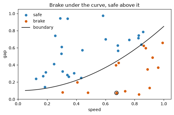
Speed across, gap to the lead car up. Some moments are safe. Some need the brake. The safe region bends: the gap you need grows with the square of speed. A straight cut through this cloud misses the pocket of brake points tucked under that bend.
The dumb rule, before any weights, is to say the common answer every time.
Predict: are more of these moments safe, or brake? Does the first moment sit under the curve?
data = generate_driving_dataset(num_samples=40, seed=42)
safe = sum(1 for _, label in data if label > 0)
brake = sum(1 for _, label in data if label < 0)
speed0, gap0 = data[0][0]
label0 = data[0][1]
speed_coef = 0.75
gap_offset = 0.1
curve0 = speed_coef * (speed0 ** 2) + gap_offset

print(len(data))
print(safe)
print(brake)
print(f"{100.0 * safe / len(data):.1f}")

safe_s, safe_g, brake_s, brake_g = [], [], [], []
for (speed, gap), label in data:
    if label > 0:
        safe_s.append(speed)
        safe_g.append(gap)
    else:
        brake_s.append(speed)
        brake_g.append(gap)
curve_s = [i / 100 for i in range(5, 101)]
curve_g = [speed_coef * s * s + gap_offset for s in curve_s]

keep_inline()
fig, ax = plt.subplots(figsize=(6, 4))
ax.scatter(safe_s, safe_g, c="#2c7fb8", s=28, label="safe")
ax.scatter(brake_s, brake_g, c="#d95f0e", s=28, label="brake")
ax.plot(curve_s, curve_g, color="#222222", lw=1.5, label="boundary")
ax.scatter([speed0], [gap0], s=80, facecolors="none", edgecolors="#222222", linewidths=1.4, zorder=3)
ax.set_xlim(0, 1.05)
ax.set_ylim(0, 1.05)
ax.set_xlabel("speed")
ax.set_ylabel("gap")
ax.set_title("Brake under the curve, safe above it")
ax.legend(frameon=False)
plt.tight_layout()
plt.show()

print(f"{speed_coef:.2f}")
print(f"{gap_offset:.1f}")
print(f"{speed0:.4f}")
print(f"{gap0:.4f}")
print(f"{curve0:.4f}")
print(label0)
40
25
15
62.5
0.75
0.1
0.6755
0.0738
0.4422
-1.0
40 moments. 25 are safe and 15 need the brake. Always saying safe is right 62.5 percent of the time, and it never touches the pedal.
The curve on the plot is 0.75 times the square of speed, plus 0.1. You saw the bend before the formula. The formula is only the rule that painted the labels. The ringed point is the first moment: speed 0.6755, gap 0.0738, label -1.0. The curve there is 0.4422. The gap is under it, so this moment is a brake. Hold 62.5 and 15. The walk has to be read against that constant rule, and against the moments the constant rule misses.
Now walk a small network over those same 40 moments. The loss is a hinge: a penalty that is zero once the prediction is far enough on the correct side of the label, and that grows when the prediction is on the wrong side. An epoch is one pass. The step size is the one the course trainer uses.
Predict: the mean hinge should walk down. Does accuracy pull away from always saying safe, or does the brake row get left behind?
epochs = 35
learning_rate = 0.08
seed = 42
random.seed(seed)
dataset = generate_driving_dataset(num_samples=40, seed=seed)
model = MLP(nin=2, nouts=[8, 8, 1], activations=["tanh", "tanh", "linear"])

losses, accs = [], []
safe_hinge, brake_hinge = [], []
last_rows = []
first_min = None

for epoch in range(1, epochs + 1):
    total_loss = Value(0.0)
    correct = 0
    safe_sum = 0.0
    brake_sum = 0.0
    safe_n = 0
    brake_n = 0
    epoch_rows = []
    epoch_min = None
    for features, label in dataset:
        pred = model(features)
        margin = Value(1.0) - (Value(label) * pred)
        loss_i = margin.relu()
        total_loss = total_loss + loss_i
        epoch_rows.append((pred.data, label))
        if epoch_min is None or pred.data < epoch_min:
            epoch_min = pred.data
        if label > 0:
            safe_sum += loss_i.data
            safe_n += 1
        else:
            brake_sum += loss_i.data
            brake_n += 1
        if (pred.data > 0 and label > 0) or (pred.data < 0 and label < 0):
            correct += 1
    loss = total_loss / len(dataset)
    losses.append(loss.data)
    accs.append(100.0 * correct / len(dataset))
    safe_hinge.append(safe_sum / safe_n)
    brake_hinge.append(brake_sum / brake_n)
    if epoch == 1:
        first_min = epoch_min
    if epoch == epochs:
        last_rows = epoch_rows
    model.zero_grad()
    loss.backward()
    for p in model.parameters():
        p.data -= learning_rate * p.grad

down = sum(losses[i + 1] < losses[i] for i in range(len(losses) - 1))
n_pos = sum(1 for pred, _ in last_rows if pred > 0)
n_neg = sum(1 for pred, _ in last_rows if pred < 0)
brake_rows = [(pred, label) for pred, label in last_rows if label < 0]
brake_hits = sum(1 for pred, _ in brake_rows if pred < 0)
end_preds = [pred for pred, _ in last_rows]

print(f"{losses[0]:.4f}")
print(f"{losses[-1]:.4f}")
print(f"{accs[0]:.1f}")
print(f"{accs[-1]:.1f}")

print(f"{safe_hinge[0]:.4f}")
print(f"{safe_hinge[-1]:.4f}")
print(f"{brake_hinge[0]:.4f}")
print(f"{brake_hinge[-1]:.4f}")

keep_inline()
fig, ax = plt.subplots(figsize=(6.2, 3.6))
xs = list(range(1, len(losses) + 1))
ax.plot(xs, losses, color="#222222", lw=2.0, label="mean")
ax.plot(xs, safe_hinge, color="#2c7fb8", lw=1.6, label="safe rows")
ax.plot(xs, brake_hinge, color="#d95f0e", lw=1.6, label="brake rows")
ax.set_xlabel("epoch")
ax.set_ylabel("hinge")
ax.set_title("The mean walks down. The brake rows do not.")
ax.legend(frameon=False)
plt.tight_layout()
plt.show()

print(down)
print(len(losses) - 1)
print(len(losses))
print(f"{learning_rate:.2f}")
print(n_pos)
print(n_neg)
print(brake_hits)
print(len(brake_rows))
print(f"{(brake_hits / len(brake_rows)):.1f}")
print(f"{first_min:.4f}")
print(f"{min(end_preds):.4f}")
print(f"{max(end_preds):.4f}")

buf = io.StringIO()
with redirect_stdout(buf):
    train(epochs=35, learning_rate=0.08, seed=42)
train_log = buf.getvalue()
print(train_log)
same_walk = ("0.9980" in train_log) and ("0.6516" in train_log)
print(same_walk)
assert same_walk
0.9980
0.6516
60.0
62.5
0.9570
0.0596
1.0664
1.6383
34
34
35
0.08
40
0
0
15
0.0
-0.0048
0.4206
1.4035
====================================================================
🚀 TRAINING 2-LAYER MLP FROM RAW SCRATCH (AUTOGRAD ENGINE)
Total Parameters: 105 | Epochs: 35 | LR: 0.08
====================================================================
Epoch 01/35 | Loss: 0.9980 | Accuracy:  60.0% | ||∇L||: 0.5870
Epoch 10/35 | Loss: 0.7451 | Accuracy:  62.5% | ||∇L||: 0.3785
Epoch 20/35 | Loss: 0.7045 | Accuracy:  62.5% | ||∇L||: 0.2068
Epoch 30/35 | Loss: 0.6704 | Accuracy:  62.5% | ||∇L||: 0.2133
Epoch 35/35 | Loss: 0.6516 | Accuracy:  62.5% | ||∇L||: 0.2252
====================================================================
✅ Training complete. The network has learned the non-linear safe braking boundary.

True
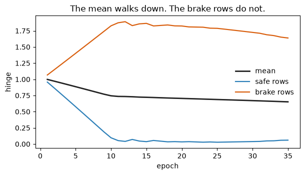
The mean hinge walks from 0.9980 to 0.6516, lower on 34 of 34 steps, across 35 epochs with step size 0.08. The dark line looks like a success. Accuracy moves from 60.0 to 62.5 and stops on the always-safe rate from the cloud.
Split the same hinge. That is the weird part, and it is the whole lesson. Safe rows go from 0.9570 to 0.0596. They go quiet. Brake rows go from 1.0664 to 1.6383. They get worse. 25 safe rows against 15 brake rows means the quiet majority pulls the average down while the brake penalty climbs. The orange line is that climb.
At the first pass the lowest score is -0.0048, a hair on the brake side of zero. By the last pass every score is positive: 40 positive, 0 negative, from 0.4206 up to 1.4035. Brake recall is 0.0, which is 0 of those 15 brake moments. The network did not learn the curve. It learned to say safe more loudly, and the moments that needed the pedal paid for that confidence.
The course trainer ends by saying the boundary was learned. It reports the same two losses, 0.9980 and 0.6516. The orange line and the 0 negative scores are the numbers to trust. A car watching only the dark line would ship this. A car that needed the brake would not.
That picture is the destination. The rest of the notebook peels the walk apart.
2. A number that remembers its parents
Multiply two typed numbers. On paper the story ends at the product. In this engine the product keeps the two numbers that made it. Those are its parents. The operation is the kind of step. Without parents, a later walk has nowhere to go.
Predict: the product remembers who made it. Does it already carry a slope?
a = Value(2.0, label="a")
b = Value(-3.0, label="b")
product = a * b
parents = sorted(p.data for p in product._prev)
print(f"{product.data:.1f}")
print(len(product._prev))
print(f"{product.grad:.1f}")
print(f"{parents[0]:.1f}")
print(f"{parents[1]:.1f}")
-6.0
2
0.0
-3.0
2.0
The product is -6.0. It has 2 parents, -3.0 and 2.0, and the gradient is still 0.0. The memory is there. The blame is not. Nobody has asked how this number should move. A car cannot steer from a memory alone. It needs a slope, and the slope stays empty until something walks backward.
3. A slope that misses the nudge
Square a sum, then ask how the square moves when only the first parent moves. The obvious slope of "something squared" is twice that something. That slope forgets that the inside of the square depends on the parent you moved.
A nudge moves that parent a hair in both directions and watches the square change. If the formula is the true slope, the nudge agrees.
Predict: will the obvious slope agree with the nudge?
a_data, b_data, c_data = 2.0, -3.0, 0.5
u = a_data * b_data + c_data
L = u ** 2
wrong = 2 * u
eps = 1e-5

def loss_at(a_value):
    return (a_value * b_data + c_data) ** 2

numeric = (loss_at(a_data + eps) - loss_at(a_data - eps)) / (2 * eps)
gap = abs(wrong - numeric)

print(f"{a_data:.1f}")
print(f"{b_data:.1f}")
print(f"{c_data:.1f}")
print(f"{u:.1f}")
print(f"{L:.2f}")
print(f"{wrong:.1f}")
print(f"{numeric:.1f}")
print(f"{gap:.1f}")

xs = [1 + i * 0.05 for i in range(41)]
bowl = [loss_at(x) for x in xs]
nudge_line = [L + numeric * (x - a_data) for x in xs]
wrong_line = [L + wrong * (x - a_data) for x in xs]

keep_inline()
fig, ax = plt.subplots(figsize=(6.2, 3.6))
ax.plot(xs, bowl, color="#222222", lw=2.0, label="the square")
ax.plot(xs, nudge_line, color="#2c7fb8", lw=1.6, label="nudge")
ax.plot(xs, wrong_line, color="#d95f0e", lw=1.6, label="obvious slope")
ax.scatter([a_data], [L], c="#222222", zorder=3)
ax.set_xlabel("a")
ax.set_ylabel("L")
ax.set_title("The obvious slope leans the wrong way")
ax.legend(frameon=False)
plt.tight_layout()
plt.show()
2.0
-3.0
0.5
-5.5
30.25
-11.0
33.0
44.0
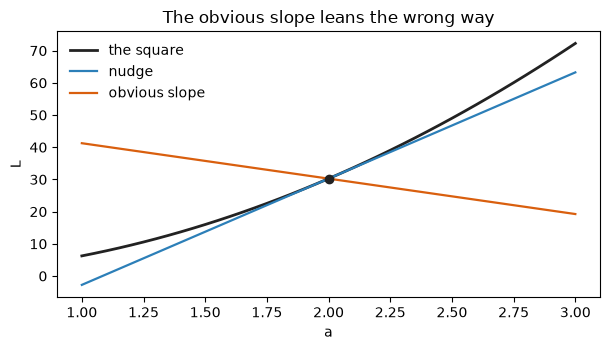
a, b, and c are 2.0, -3.0, and 0.5. The inside is -5.5. The square L is 30.25. The obvious slope, twice that inside, is -11.0. The nudge is 33.0. They miss by 44.0.
The plot is the disagreement. The black curve is the square. The blue line is the nudge, and it follows the curve through the dot. The orange line is the obvious slope: shallower, and leaning the other way. Twice the inside is the slope with respect to the inside. The parent you moved still has to be allowed to change that inside. A brake controller with the orange slope would turn the wheel the wrong amount. The link that was dropped is b.
4. Blame flows backward
The chain rule is blame, handed backward. The final number starts with the slope of a number with respect to itself. Each parent receives that blame times how strongly the parent affected the child. At a multiply, the strength is the other parent's value. At an add, the child passes the blame along unchanged. At a square, the strength is twice the inside. Multiply those strengths along the path and you recover the nudge. You do not rewrite the algebra. The parents already stored the path.
Predict: after the walk, does a's blame match the nudge from the plot above?
a = Value(a_data, label="a")
b = Value(b_data, label="b")
c = Value(c_data, label="c")
u_node = a * b + c
loss = u_node ** 2
loss.backward()
print(f"{loss.grad:.1f}")
print(f"{a.grad:.1f}")
print(f"{b.grad:.1f}")
print(f"{c.grad:.1f}")
print(f"{(b.data * wrong):.1f}")
1.0
33.0
-22.0
-11.0
33.0
The walk starts with blame 1.0 on L. a receives 33.0, the same nudge as the blue line. b receives -22.0. c receives -11.0, which is the orange slope we tried to give to a. The missing factor was the other parent: b is -3.0, and -3.0 times -11.0 is 33.0. The graph did the multiplication because it remembered the parents. For a car, this is the difference between a slope you hoped was right and a slope that survives a nudge.
One parent can be used twice. Square a number by multiplying it by itself. The parent set stores that object once. The multiply still counts both uses, and the blame adds.
Predict: one object in the parent set. Does the slope count one use, or both? What happens if you walk backward a second time without clearing?
x = Value(3.0, label="x")
y = x * x
print(f"{x.data:.1f}")
print(f"{y.data:.1f}")
print(len(y._prev))
y.backward()
print(f"{x.grad:.1f}")
y.backward()
print(f"{x.grad:.1f}")
3.0
9.0
1
6.0
12.0
x is 3.0 and y is 9.0, with 1 parent in the set. The first walk gives x a slope of 6.0. That is both uses added, 3.0 plus 3.0. The second walk, with the old slope still sitting there, gives 12.0. Blame adds. A leftover gradient is a second, unwanted correction. Training clears the slope before every walk for this reason. On a car, a leftover slope is a steering command applied twice.
5. A gate stuck shut
ReLU keeps a positive number and turns every other number into zero. Picture a gate. Open, blame walks through unchanged. Shut, the output is zero and so is the blame. Earlier parents learn nothing. The gate is stuck shut. That is a dead ReLU.
Put the gate on a sum. One choice of parents drives the sum negative. Another drives it positive.
Predict: which sum passes blame back to its parents, the negative one or the positive one?
shut_in = Value(-1.5)
shut = shut_in.relu()
shut.backward()
open_in = Value(1.5)
opened = open_in.relu()
opened.backward()
print(f"{shut_in.data:.1f}")
print(f"{shut.data:.1f}")
print(f"{shut_in.grad:.1f}")
print(f"{open_in.data:.1f}")
print(f"{opened.data:.1f}")
print(f"{open_in.grad:.1f}")

dead_a, dead_b, dead_c = Value(2.0), Value(-1.0), Value(1.0)
dead_pre = dead_a * dead_b + dead_c
dead = dead_pre.relu()
dead.backward()
live_a, live_b, live_c = Value(2.0), Value(1.0), Value(1.0)
live_pre = live_a * live_b + live_c
live = live_pre.relu()
live.backward()
print(f"{dead_pre.data:.1f}")
print(f"{dead.data:.1f}")
print(f"{dead_a.grad:.1f}")
print(f"{dead_b.grad:.1f}")
print(f"{dead_c.grad:.1f}")
print(f"{live_pre.data:.1f}")
print(f"{live.data:.1f}")
print(f"{live_a.grad:.1f}")
print(f"{live_b.grad:.1f}")
print(f"{live_c.grad:.1f}")

keep_inline()
labels = ["a", "b", "c"]
dead_g = [dead_a.grad, dead_b.grad, dead_c.grad]
live_g = [live_a.grad, live_b.grad, live_c.grad]
xpos = [0, 1, 2]
width = 0.36
fig, ax = plt.subplots(figsize=(6.2, 3.6))
ax.bar([i - width / 2 for i in xpos], dead_g, width=width, color="#bdbdbd", label="shut")
ax.bar([i + width / 2 for i in xpos], live_g, width=width, color="#2c7fb8", label="open")
ax.axhline(0, color="#888888", lw=0.8)
ax.set_xticks(xpos, labels)
ax.set_ylabel("blame")
ax.set_title("A shut gate passes no blame")
ax.legend(frameon=False)
plt.tight_layout()
plt.show()
-1.5
0.0
0.0
1.5
1.5
1.0
-1.0
0.0
0.0
0.0
0.0
3.0
3.0
1.0
2.0
1.0
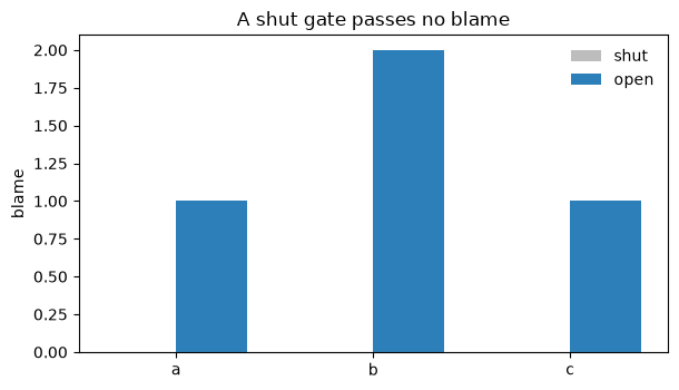
On a bare ReLU, input -1.5 becomes output 0.0 with slope 0.0. Input 1.5 stays 1.5 with slope 1.0. The first gate is shut. The second is open.
Through a sum, the shut case is worse, because the silence spreads. The pre-activation is -1.0, the output is 0.0, and parents a, b, and c all receive 0.0. Three gray bars. Nobody learns. The open case has pre-activation 3.0 and output 3.0, and the slopes are 1.0, 2.0, and 1.0. Blame got through: the gate's own slope is 1.0, and parent b still multiplies a's share, which is why a gets 1.0 while b gets 2.0. Same walk as the square, with an extra door.
A dead unit in a brake network is a sensor that has stopped teaching. The plot is the whole fact.
6. The knobs that walked
The walk in the first picture was this same machine, stacked. A neuron is a weighted sum, plus a bias, then a bend. The toy uses tanh for the bends. tanh squashes any real number toward a ceiling, and its slope fades as the output presses against that ceiling. That fade is a softer version of the shut gate: the number is still there, and the blame is almost gone.
Predict: a moderate input still has a slope. Does a large input?
for raw in (2.0, 8.0):
    node = Value(raw)
    bent = node.tanh()
    bent.backward()
    print(f"{raw:.1f}")
    print(f"{bent.data:.4f}")
    print(f"{node.grad:.4f}")
2.0
0.9640
0.0707
8.0
1.0000
0.0000
tanh of 2.0 is 0.9640, and the slope is 0.0707. Already near the ceiling, still a little blame. tanh of 8.0 is 1.0000, and the slope is 0.0000. The output has arrived and the parents will not hear about it. A shut ReLU and a tanh pressed flat are the same kind of silence. One of them is a hard zero. The other is a number that looks decided and teaches nothing.
Count the knobs in the toy that walked the hinge. Each layer is weights plus one bias per neuron.
Predict: where do most of the knobs sit, the first layer or the middle?
random.seed(0)
net = MLP(nin=2, nouts=[8, 8, 1], activations=["tanh", "tanh", "linear"])
counts = [len(layer.parameters()) for layer in net.layers]
print(len(net.layers[0].neurons[0].w))
print(len(net.layers[0].neurons))
print(len(net.layers[1].neurons))
print(len(net.layers[2].neurons))
print(counts[0])
print(counts[1])
print(counts[2])
print(len(net.parameters()))
2
8
8
1
24
72
9
105
Two inputs, then 8 neurons, then 8, then 1 readout. The layers hold 24 knobs, then 72, then 9. Together that is 105, the length of the parameter list. Most of the memory is the middle layer: 72 of those 105. The hinge that walked from 0.9980 to 0.6516 was these 105 numbers taking steps of 0.08. Enough knobs to bend with the curve. They spent the steps getting louder about safe instead.
7. Your turn
Exercise — local slope of a square. Inside Value.__pow__, the local factor is power * x ** (power - 1), then times the blame coming from upstream. Leave the TODO as it is to use the reference. If solutions/00_nn_scratch/exercises.py defines power_rule_grad, the cell uses that instead.
Predict: for a square, you already watched a parent used twice. Which slope should come back?
def power_rule_grad_student(x, power, upstream):
    # TODO: power * x ** (power - 1) * upstream
    raise NotImplementedError("TODO")

def reference_power_rule_grad(x, power, upstream):
    return (power * (x ** (power - 1))) * upstream

def load_exercises():
    path = REPO / "solutions" / "00_nn_scratch" / "exercises.py"
    print("solutions file exists:", path.is_file())
    if not path.is_file():
        return None
    spec = importlib.util.spec_from_file_location("nn_exercises", path)
    mod = importlib.util.module_from_spec(spec)
    spec.loader.exec_module(mod)
    return mod

exercise_mod = load_exercises()

def resolve(student, name, reference, probe):
    try:
        student(*probe)
    except NotImplementedError:
        if exercise_mod is not None and hasattr(exercise_mod, name):
            print("using solution", name)
            return getattr(exercise_mod, name)
        print("using reference", name)
        return reference
    print("using yours", name)
    return student

power_fn = resolve(power_rule_grad_student, "power_rule_grad", reference_power_rule_grad, (3.0, 2, 1.0))
x_probe, power, upstream = 3.0, 2, 1.0
got = power_fn(x_probe, power, upstream)
check_x = Value(x_probe)
(check_x ** power).backward()
print(f"{x_probe:.1f}")
print(power)
print(f"{upstream:.1f}")
print(f"{got:.1f}")
print(f"{check_x.grad:.1f}")
assert abs(got - check_x.grad) < 1e-9
print("✅", got)
solutions file exists: False
using reference power_rule_grad
3.0
2
1.0
6.0
6.0
✅ 6.0
The cell ends with ✅. The square of 3.0, with upstream blame 1.0 and power 2, has slope 6.0. That is the same 6.0 as the parent that was used twice: both uses added. The reference ran because the TODO still raises. There is no solutions file for this appendix on the course tree, so the reference is the fallback. Replace the TODO and run the cell again if you want the check to call your function.
Solution
return (power * (x ** (power - 1))) * upstream
Exercise — the gate. Return 0 when the input is not positive. Otherwise return the upstream blame unchanged. Same rule as Value.relu: a zero input stays shut. Leave the TODO in place to use the reference. A solutions file, if present, should define relu_gate.
Predict: which of the two inputs from the bar chart returns the upstream blame unchanged?
def relu_gate_student(x, upstream):
    # TODO: 0 when x is not positive, otherwise the upstream blame
    raise NotImplementedError("TODO")

def reference_relu_gate(x, upstream):
    return (1.0 if x > 0.0 else 0.0) * upstream

gate_fn = resolve(relu_gate_student, "relu_gate", reference_relu_gate, (-1.5, 1.0))
for raw, up in ((-1.5, 1.0), (1.5, 1.0)):
    got = gate_fn(raw, up)
    node = Value(raw)
    node.relu().backward()
    print(f"{raw:.1f}")
    print(f"{up:.1f}")
    print(f"{got:.1f}")
    print(f"{node.grad:.1f}")
    assert abs(got - node.grad) < 1e-9
print("✅", gate_fn(-1.5, 1.0), gate_fn(1.5, 1.0))
using reference relu_gate
-1.5
1.0
0.0
0.0
1.5
1.0
1.0
1.0
✅ 0.0 1.0
The cell ends with ✅. Input -1.5 with upstream blame 1.0 returns 0.0. Input 1.5 returns 1.0. Shut, then open. The same two facts as the gray bars and the blue bars. The reference ran because the TODO still raises. Replace the TODO and run the cell again if you want the check to call your function.
Solution
if x > 0.0:
    return upstream
return 0.0
8. Recap
- A typed 1.5 has gradient 0.0 and 0 parents. The product -6.0 remembers 2 parents, -3.0 and 2.0, and still has gradient 0.0 until a walk asks.
- Squaring the sum gave L = 30.25 from an inside of -5.5. The obvious slope was -11.0. The nudge was 33.0. They miss by 44.0. The orange tangent leans the wrong way.
- Blame starts at 1.0. The walk assigned 33.0, -22.0, and -11.0. The orange number times the other parent, -11.0 times -3.0, is the nudge. The parents stored that product.
- Using 3.0 twice stored 1 parent and a slope of 6.0. A second walk without a clear made 12.0. Blame adds, which is why training clears the slope.
- ReLU on -1.5 is output 0.0 and slope 0.0. On 1.5 the output is 1.5 and the slope is 1.0. Through the shut sum, three parents got 0.0. Through the open sum the slopes were 1.0, 2.0, and 1.0.
- tanh of 8.0 is 1.0000 with slope 0.0000. tanh of 2.0 is 0.9640 with slope 0.0707. A ceiling can silence blame while the output still looks decided.
- The toy has 105 knobs: 24, then 72, then 9. The mean hinge walked from 0.9980 to 0.6516, down on 34 of 34 steps. Accuracy ended at 62.5, the always-safe rate on 25 of 40 moments. Safe rows went quiet, 0.9570 to 0.0596. Brake rows got worse, 1.0664 to 1.6383. Brake recall was 0.0, 0 of 15, and all 40 final scores were positive. A falling mean is not a learned boundary.
Go deeper
- Karpathy — micrograd is the scalar engine this
Valueclass follows. - Neural Networks: Zero to Hero, lecture 1 builds that engine on video. The series index is karpathy.ai/zero-to-hero.
- 3Blue1Brown — Backpropagation draws the same blame walking backward.