Week 3: Your first perception box

What you will be able to do

Turn an image row into a distance ahead on a flat road, and explain why one pixel column covers more ground the further away it is
Proof Practice problems 1 and 2 in the lab, and the quiz questions on the horizon, row distances and metres per column
Estimate the car's offset and heading from paint masks with two lane-centre points and a straight line, and report no estimate when the paint is missing
Proof Your estimate_lane passes the Exercise A check in the lab
Drive the car on your own perception, and explain why a straight-line lane model is biased on bends and why a flipped sign drives the car off the road
Proof Your estimate_lane passes the Exercise B check, the straight-roads and break-it sections of the lab, and the quiz questions on bends and signs

Warm-up review

Nothing is due today. Pass a week's quiz and its questions come back here at growing intervals.

Lecture

The horizon

Your paint_masks from unit 0.1.2 finds the paint pixels, but the controller wants two numbers: how far the car is from lane centre in metres (the offset, positive when left of centre) and which way it points relative to the lane in radians (the heading, positive when pointing left of the lane). This unit builds the box in between, estimate_lane(obs), which returns a LaneEstimate(offset_m, heading_rad, valid).

The bridge from pixels to metres is one assumption. A 2008 lane-detection paper states it in its first step:

"To get the IPM of the input image, we assume a flat road, and use the camera intrinsic (focal length and optical center) and extrinsic (pitch angle, yaw angle, and height above ground) parameters to perform this transformation." (Aly, 2008, §II.A)

IPM, inverse perspective mapping, redraws the picture as if seen from straight above, so "lanes that appear to converge at the horizon line are now vertical and parallel." You will do it for just the pixels you need.

In this flat-world teaching simulator the ground is exactly a plane, and you know every camera number. The camera sits $h = 1.4$ m above the ground, directly above the front axle, tipped down by a pitch of $p = 5°$ . Its focal length is $f = 160$ pixels: a ray at angle $\alpha$ from the direction the camera points lands $f \tan\alpha$ pixels from the image centre, which is column $c_x = 159.5$ , row $c_y = 89.5$ .

The horizon is where a ray parallel to the ground lands. That ray points 5° above the camera's axis, so it lands $f \tan 5° = 160 \times 0.0875 = 14.0$ rows above the centre: row $89.5 - 14.0 = 75.5$ . Rows above it see sky, which is why rows 0 to 75 of the 0.1.2 frame were all sky.

How we got row 75.5

The camera's axis points $p = 5°$ below horizontal, so a ray that runs parallel to the ground is $5°$ above the axis. The rule from above says a ray at angle $\alpha$ from the axis lands $f\tan\alpha$ pixels from the image centre. With $\alpha = 5°$ , a calculator gives $\tan 5° = 0.0875$ , so

f\tan 5° = 160 \times 0.0875 = 14.0 \text{ pixels}

The ray points above the axis, so it lands above the centre. Row numbers count downwards from the top of the picture, so going up means subtracting: $c_y - 14.0 = 89.5 - 14.0 = 75.5$ .

Rows are distances

Take a row $v$ below the horizon. Its ray points $\arctan\frac{v - c_y}{f}$ below the camera's axis, and the axis points $p$ below horizontal, so the ray falls at

\theta = p + \arctan\frac{v - c_y}{f}

below horizontal. It starts at height $h$ and meets the ground a distance $d$ ahead: a right-angled triangle with $\tan\theta = h / d$ , so

d = \frac{h}{\tan\theta}

Figure 1. Left: side view of rays for five rows meeting the ground 2.06 to 11.45 m ahead. Right: distance ahead against row, rising steeply towards the horizon at row 75.5.

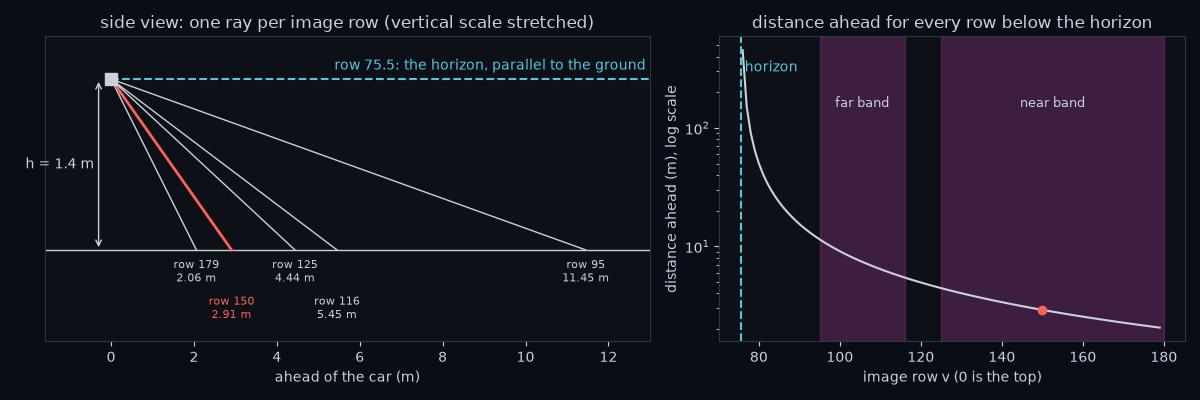
Worked example. How far ahead is the ground seen in row 150?

$(150 - 89.5) / 160 = 0.378$ , and $\arctan 0.378 = 20.71°$ .
$\theta = 5° + 20.71° = 25.71°$ , and $\tan 25.71° = 0.4815$ .
$d = 1.4 / 0.4815 = 2.91$ m.

The column never appears in the formula: every pixel in row 150 sees ground 2.91 m ahead. A row is a distance.

Camera.pixel_to_ground(u, v) does this for you: it takes a column $u$ and a row $v$ and returns the ground point (forward, left) in metres from the camera, left positive, or NaN (not a number) above the horizon. The lab checks the worked example against it; module 1.4 opens it up.

The distances are uneven: at the bottom one row is 2 cm of road, near row 100 it is 36 cm, and five rows below the horizon you are past 50 m. Rows near the horizon are too coarse to trust, so the box measures in two bands: the near band, rows 125 to 179 (2.1 to 4.4 m ahead), and the far band, rows 95 to 115 (5.6 to 11.5 m).

How we got the row sizes and band distances

Each number is the row formula from the worked example, $\theta = p + \arctan\frac{v - c_y}{f}$ and then $d = h / \tan\theta$ , applied to one more row $v$ (with $p = 5°$ , $c_y = 89.5$ , $f = 160$ and $h = 1.4$ m):

row $v$	$\theta$	$\tan\theta$	$d = 1.4 / \tan\theta$
179	34.22°	0.6801	2.058 m
178	33.95°	0.6732	2.080 m
125	17.51°	0.3155	4.438 m
115	14.06°	0.2504	5.592 m
101	9.11°	0.1604	8.730 m
100	8.75°	0.1540	9.091 m
95	6.97°	0.1222	11.454 m
80	1.60°	0.0280	50.057 m

Each $d$ is worked out from unrounded values, so dividing the rounded columns can differ in the last digit. Reading off the table:

The near band runs from row 125 to row 179, which is 4.438 m to 2.058 m ahead: 2.1 to 4.4 m. The far band runs from row 95 to row 115, which is 11.454 m to 5.592 m ahead: 5.6 to 11.5 m.
One row of road is the difference between neighbouring rows. At the bottom, $2.080 - 2.058 = 0.021$ m, which is 2 cm. Near row 100, $9.091 - 8.730 = 0.361$ m, which is 36 cm.
Row 80 sees ground 50.057 m ahead, past 50 m. The horizon is at row 75.5, so row 80 is only $80 - 75.5 = 4.5$ rows below it: about five.

Metres per pixel

The tempting shortcut: "The lane is 3.6 m wide. Count the columns it spans, divide, and you know the metres per column; multiply any pixel's column by it." That fails, because a pixel column is not a fixed number of metres. Sideways distances shrink with distance, just as a far-off car looks smaller.

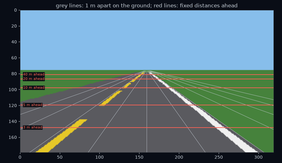
Figure 2. The straight road with lines 1 m apart on the ground, far apart at the bottom of the frame and crowding together near the horizon.

A point $L$ metres to the left and about $d$ metres ahead appears roughly $f L / d$ columns from the centre, so one column covers about

\text{metres per column} \approx \frac{d}{f}

Measured with pixel_to_ground, one column covers 0.0189 m in row 150 (2.91 m ahead), 0.0574 m in row 100 (9.09 m ahead) and 0.312 m in row 80 (50.1 m ahead), each close to $d/f$ ; the 5° pitch accounts for the differences.

Worked example. The 3.6 m lane spans $3.6 / 0.01886 = 191$ columns in row 150 but $3.6 / 0.05737 = 63$ in row 100 (the two column sizes again, with one more digit). Slide the car 0.5 m left and the white line moves $0.5 / 0.01886 = 26.5$ columns in row 150, but only $0.5 / 0.05737 = 8.7$ in row 100; the lab measures both. To turn a pixel into metres you need its row as well as its column.

From masks to a lane estimate

Offset and heading describe the lane centre, halfway between the yellow line and the white line, which are 3.6 m apart. The box finds two points on it and draws a straight line through them:

Masks: yellow, white = paint_masks(obs.frame).
Centroids: in each band, each line's centroid is the mean column and mean row of its paint pixels there. The centroid of a thin line lies on the line, so it is a point on the paint; pixel_to_ground turns it into (forward, left).
Lane centre: in each band, the midpoint of the yellow and white ground points. That gives a near point $(f_1, c_1)$ and a far point $(f_2, c_2)$ , forward first.
Line: its slope, the metres it drifts left per metre ahead, is $(c_2 - c_1) / (f_2 - f_1)$ .

At the car, forward $= 0$ , the line is at left $= c_1 - \text{slope} \cdot f_1$ ; if the lane centre is 0.4 m to the car's right, the car is 0.4 m left of the lane centre. The line points $\arctan(\text{slope})$ left of the car; if the lane points left of the car, the car points right of the lane. So

\text{offset} = -(c_1 - \text{slope} \cdot f_1), \qquad \text{heading} = -\arctan(\text{slope})

Both minus signs switch from the lane seen by the car to the car seen by the lane.

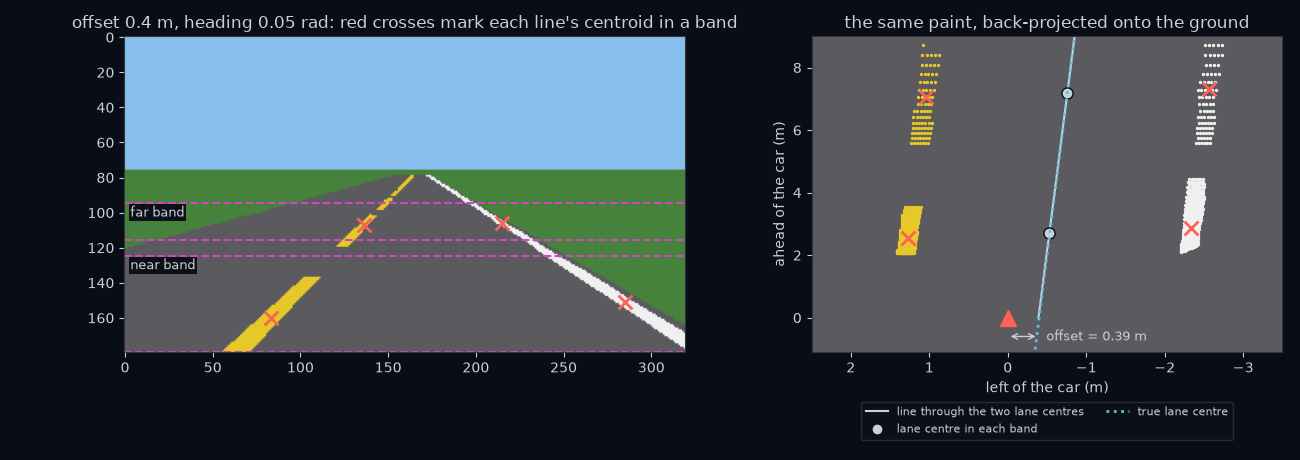
Figure 3. Left: the worked-example frame with the two bands and each line's centroid marked. Right: the same paint from above, the two lane-centre points, and the line through them passing 0.39 m right of the car.

Worked example. The car is on the straight road, truly 0.4 m left of centre and turned 0.05 rad left (the frame above).

Near band: the yellow line's 553 pixels have their centroid at column 83.02, row 159.85: ground point (2.55, 1.27). The white line's 543 pixels give (2.87, −2.33). Their midpoint, the near lane centre, is (2.71, −0.53).
Far band: yellow (99 pixels) at (7.05, 1.05), white (104 pixels) at (7.33, −2.57), lane centre (7.19, −0.76).
$\text{slope} = (-0.76 + 0.53) / (7.19 - 2.71) = -0.0512$ : the lane centre drifts right as it goes ahead.
$c_1 - \text{slope} \cdot f_1 = -0.53 + 0.0512 \times 2.71 = -0.39$ , so the offset is $+0.39$ m (truth 0.40), and the heading is $-\arctan(-0.0512) = +0.051$ rad (truth 0.05). The arithmetic uses unrounded values.

How we got the four ground points

pixel_to_ground turns a centroid (column, row) into a ground point in two parts. Take the near yellow centroid, at column 83.02 and row 159.85.

Forward. The row formula depends on the row alone:

\theta = 5° + \arctan\frac{159.85 - 89.5}{160} = 5° + 23.73° = 28.73°, \qquad d = \frac{1.4}{\tan 28.73°} = 2.55 \text{ m}

Left. The picture's centre is column 159.5, so the centroid is $159.5 - 83.02 = 76.48$ columns to its left (a column left of centre is on the car's left, so this is positive). One column in row 159.85 covers 0.01666 m: that is how far pixel_to_ground moves the ground point sideways when the column goes up by one, the measurement described in "Metres per pixel". Then

76.48 \times 0.01666 = 1.27 \text{ m}

That is the ground point $(2.55, 1.27)$ . The other three work the same way. A centroid right of the picture's centre has a negative number of columns, so it lands on the car's right:

centroid	column	row	forward	columns left of centre	metres per column	left
near yellow	83.02	159.85	2.55 m	76.48	0.01666	1.27 m
near white	284.94	151.03	2.87 m	−125.44	0.01861	−2.33 m
far yellow	136.04	106.96	7.05 m	23.46	0.04467	1.05 m
far white	214.86	105.81	7.33 m	−55.36	0.04637	−2.57 m

What valid=False is for

Sometimes there is nothing to measure: turn the car 0.6 rad left on a straight road and the white line leaves the near band: 0 pixels, so no lane centre and no line. The box counts a line as seen in a band only with at least 3 pixels there.

What should estimate_lane return then? Offset 0 and heading 0 is a lie: it tells the controller "you are perfectly centred" when you know nothing, and the controller will act on it. Return LaneEstimate(math.nan, math.nan, False). valid=False says plainly there is no estimate, and the NaNs spoil any sum that forgets to check, so the mistake shows up.

What to do then is the controller's decision: the provided controller checks valid first and, when it is False, holds the wheel straight. With the provided box on gentle, all 1,778 steps are valid.

Straight roads only

Your box fits a straight line, which is exact on a straight road: on 40 centred, aligned frames along it, every estimate is within 0.01 m and 0.003 rad. On a bend the lane centre is a curve, and a straight line through two points on a curve, a chord, does not point along the curve at the car. The estimate is wrong even when the car is placed perfectly:

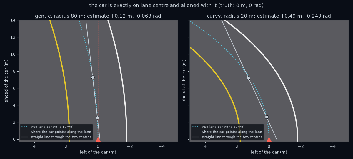
Figure 4. From above, a car exactly on lane centre on bends of radius 80 m and 20 m. The line through the two lane-centre points misses the car and leans right, much more on the tight bend.

You can predict the error. On a bend of radius $R$ turning left, the lane centre $s$ metres ahead has drifted about $s^2 / (2R)$ to the left. With the near point $s_1$ metres ahead and the far point $s_2$ , the line through them has

\text{slope} = \frac{s_2^2 - s_1^2}{2R\,(s_2 - s_1)} = \frac{s_1 + s_2}{2R}, \qquad \text{left at the car} = -\frac{s_1 s_2}{2R}

so the box reports an offset of $s_1 s_2 / (2R)$ and a heading of $-\arctan\frac{s_1 + s_2}{2R}$ where both should be 0. With $s_1 \approx 2.7$ m and $s_2 \approx 7.2$ m, that predicts errors of 0.12 m and 0.062 rad on gentle ( $R = 80$ m) and 0.49 m and 0.24 rad on curvy ( $R = 20$ m). On 40 centred frames in each road's bends, the median errors are 0.13 m and 0.065 rad on gentle, as predicted, and 0.60 m and 0.30 rad on curvy: there, your lane's radius is only 18.2 m on right bends, and the far midpoint sits about 0.1 m inside the lane centre.

How we got 0.12 m, 0.062 rad, 0.49 m and 0.24 rad

Put the numbers into the two formulas above: $s_1 = 2.7$ m and $s_2 = 7.2$ m are how far ahead the near and far points are, and $R$ is the bend radius. The predicted offset is $s_1 s_2 / (2R)$ . The predicted heading is the angle whose tangent is the slope $(s_1 + s_2) / (2R)$ , and $\arctan$ gives that angle in radians.

On gentle, $R = 80$ m:

\text{offset} = \frac{2.7 \times 7.2}{2 \times 80} = \frac{19.44}{160} = 0.1215 \approx 0.12 \text{ m}

\text{slope} = \frac{2.7 + 7.2}{2 \times 80} = \frac{9.9}{160} = 0.0619, \qquad \text{heading} = \arctan 0.0619 = 0.0618 \approx 0.062 \text{ rad}

On curvy, $R = 20$ m:

\text{offset} = \frac{19.44}{2 \times 20} = 0.486 \approx 0.49 \text{ m}

\text{slope} = \frac{9.9}{2 \times 20} = 0.2475, \qquad \text{heading} = \arctan 0.2475 = 0.2426 \approx 0.24 \text{ rad}

The slope is 0.2475, but the heading is the angle, and for a slope this big the angle is a little smaller than the slope.

How we got 18.2 m

The bends of curvy have radius 20 m along the road's centre line, the yellow line. Your lane's centre is 1.8 m to the right of that line. A right bend turns towards the right, so your lane is on the inside of the turn, and a circle on the inside is smaller:

20 - 1.8 = 18.2 \text{ m}

On a left bend your lane is on the outside, so the radius is $20 + 1.8 = 21.8$ m. Putting $R = 18.2$ into the formulas above instead of 20 raises the predicted errors from 0.49 m and 0.24 rad to $19.44 / 36.4 = 0.53$ m and $\arctan(9.9 / 36.4) = 0.27$ rad; with 21.8 they fall to 0.45 m and 0.22 rad.

This is a bias, not noise: on a left bend the box always says "left of centre, pointing right", so the controller steers further left and the car cuts to the inside. That is why the grader tests your function on straight roads only: none of those bend frames falls within its tolerances of 0.25 m and 0.05 rad. Better lane models fit curves through many rows; that is module 1.5, "Classical lane perception". Unit 0.1.4 shows what this bias does to the car on curvy.

Swap your perception into the car

Car(perception=estimate_lane) is the provided car with your perception inside: every 0.05 s it calls your function with an Observation holding the camera frame obs.frame, the speed obs.speed and the time obs.t.

Check 0.1.3.b drives that car around gentle: it must complete the lap with a mean lateral error below 0.5 m (the provided box manages 0.38 m), and it refuses a car still running the provided perception.

One flipped sign turns a working box into a dangerous one. With the offset's sign wrong, the car believes it is left of centre when it is right, and steers away from the centre; each correction makes the error bigger, and the bigger error a bigger wrong correction. This is positive feedback. In the lab the error roughly doubles every half second until the car leaves the lane after 5 s, still on the first straight.

Go deeper

Stanford CS231A Course Notes 1, "Camera Models" (Hata and Savarese), §2 "Pinhole cameras": the similar triangles behind $f L / d$ .
Aly, "Real time Detection of Lane Markers in Urban Streets" (2008), §II.A "Inverse Perspective Mapping (IPM)" and Figures 2 and 3: the flat-road top view of a real street. The rest can wait for module 1.5.
Szeliski, "Computer Vision: Algorithms and Applications" (2nd ed.), §2.1.4 "3D to 2D projections", subsections "Perspective" and "Camera intrinsics". A graduate textbook (free after a short form); keep it for module 1.4.

Go deeper

Playground

Open full tab

Lab

Write the box in Colab and run its checks. Come back here for the quiz.

Open lab in Colab

Checkpoint quiz

Teach it back

Explain this week as if to a friend who has never seen it. Then paste it, with the prompt below, into any AI tutor and ask it to find the gaps.

Show the tutor prompt

You are a Socratic tutor for unit 0.1.3 "Your first perception box" of a self-driving car course. I am a programmer with rusty maths and no machine-learning background. I have just read a lecture and done a lab on turning a camera frame into the car's position in its lane.

What the unit taught (use these facts exactly):
- The simulator's road is exactly flat. The camera is 1.4 m above the ground at the front axle, tipped down 5 degrees, focal length f = 160 pixels, image centre column 159.5 and row 89.5. The horizon is row 75.5.
- A row is a distance: the ray of row v falls theta = 5 degrees + arctan((v - 89.5) / 160) below horizontal and meets the ground d = 1.4 / tan(theta) metres ahead. Row 150 sees 2.91 m ahead, row 100 sees 9.09 m.
- One pixel column covers about d / f metres of ground: 0.0189 m in row 150, 0.0574 m in row 100. Sliding the car 0.5 m moves the white line 26.5 columns in row 150 but 9 in row 100.
- The box: paint masks; in a near band (rows 125 to 179) and a far band (rows 95 to 115), each line's centroid, turned into a ground point (forward, left); the lane centre is the midpoint of the yellow and white points; a straight line through the near and far lane-centre points. offset = -(c1 - slope * f1), heading = -arctan(slope). Left is positive.
- With fewer than 3 pixels of a line in a band, the box returns LaneEstimate(nan, nan, False), never 0 and 0.
- On a bend of radius R the straight line through two points is a chord: with the car centred the box reports about s1 * s2 / (2R) offset and -arctan((s1 + s2) / (2R)) heading, with s1 about 2.7 m and s2 about 7.2 m. That is 0.12 m and 0.062 rad on the 80 m bends of gentle. It is a bias, not noise.
- Misconception to probe: "a pixel column is a fixed number of metres". It is not; it grows with distance ahead.
- A flipped offset sign makes the controller steer away from the centre: positive feedback, the error roughly doubling every half second until the car leaves the road after 5 s.

How to run the session:
1. Ask me ONE question at a time, then wait for my answer. Start by asking me why every pixel in one row of the image sees ground at the same distance ahead.
2. Never give me the answer. If I am wrong or vague, ask a smaller question, or give me numbers to work through by hand, so I find the mistake myself.
3. Within the first three questions, test the misconception: ask whether the lane's width in columns in row 150 lets me convert columns to metres in row 100, and why.
4. Ask at least one question where I compute a distance ahead for a row you give me, one where I compute an offset from two lane-centre points you give me, and one where I explain what the box reports on a bend with the car perfectly centred.
5. Keep your turns short: two or three sentences, then the question.
6. After about five exchanges, stop. List what I explained well, and what I should revisit, naming these lecture sections: "The horizon", "Rows are distances", "Metres per pixel", "From masks to a lane estimate", "What valid=False is for", "Straight roads only", "Swap your perception into the car".

Pilot log

0 logged

Saved in this browser. It tells the course author where this week is hard.

Minutes you spent on this week's workMost confusing moment (optional)

Confidence (1 = lost, 5 = could teach it)